In this notebook we’ll be implementing one of the ResNet (Residual Network) model variants. Much like the VGG model introduced in the previous notebook, ResNet was designed for the ImageNet challenge, which it won in 2015.
ResNet, like VGG, also has multiple configurations which specify the number of layers and the sizes of those layers. Each layer is made out of blocks, which are made up of convolutional layers, batch normalization layers and residual connections (also called skip connections or shortcut connections). Confusingly, ResNets use the term “layer” to refer to both a set of blocks, e.g. “layer 1 has two blocks”, and also the total number of layers within the entire ResNet, e.g. “ResNet18 has 18 layers”.
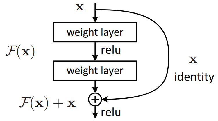
A residual connection is simply a direct connection between the input of a block and the output of a block. Sometimes the residual connection has layers in it, but most of the time it does not. Below is an example block with an identity residual connection, i.e. no layers in the residual path.

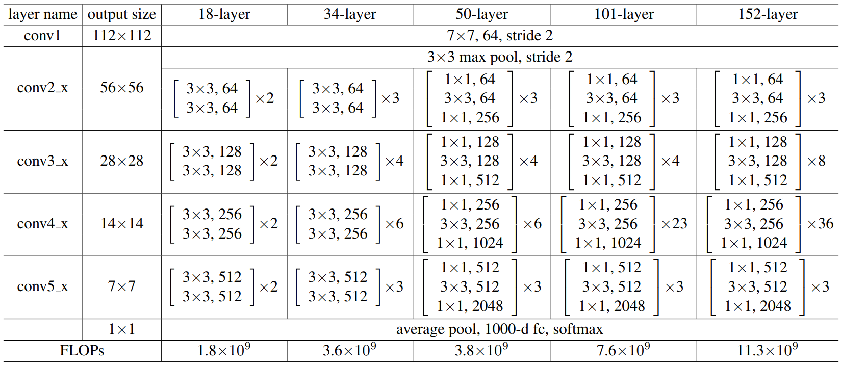
The different ResNet configurations are known by the total number of layers within them – ResNet18, ResNet34, ResNet50, ResNet101 and ResNet152.

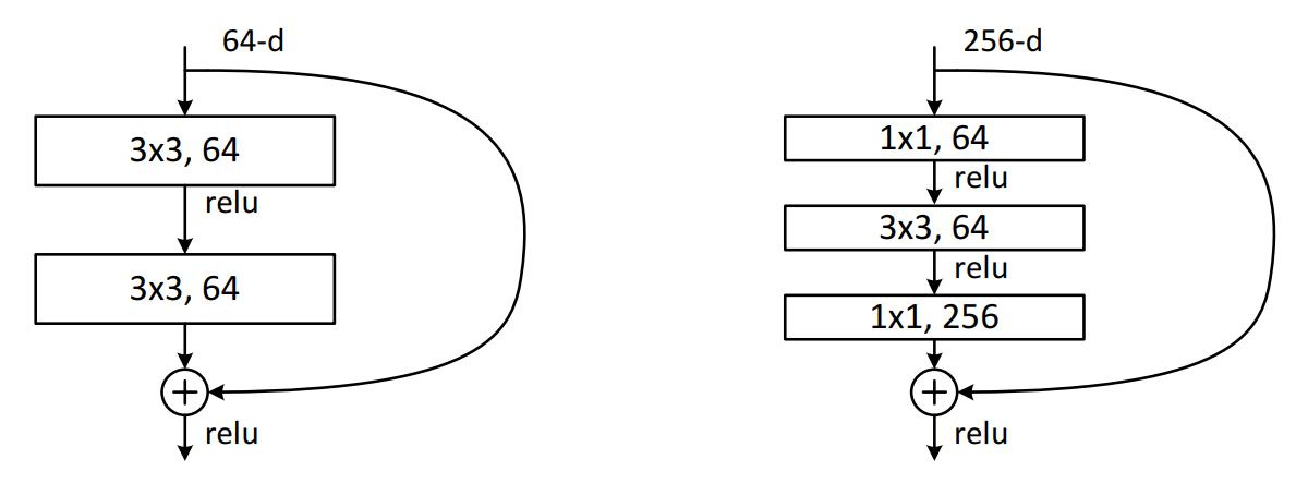
From the table above, we can see that for ResNet18 and ResNet34 that the first block contains two 3×3 convolutional layers with 64 filters, and that ResNet18 has two of these blocks in the first layer, whilst Resnet34 has three. ResNet50, ResNet101 and ResNet152 blocks have a different structure than those in ResNet18 and ResNet34, and these blocks are called bottleneck blocks. Bottleneck blocks reduce the number of number of channels within the input before expanding them back out again. Below shows a standard BasicBlock (left) – used by ResNet18 and ResNet34 – and the Bottleneck block used by ResNet50, ResNet101 and ResNet152.

Why do ResNets work? The key is in the residual connections. Training incredibly deep neural networks is difficult due to the gradient signal either exploding (becoming very large) or vanishing (becoming very small) as it gets backpropagated through many layers. Residual connections allow the model to learn how to “skip” layers – by setting all their weights to zero and only rely on the residual connection. Thus, in theory, if your ResNet152 model can actually learn the desired function between input and output by only using the first 52 layers the remaining 100 layers should set their weights to zero and the output of the 52nd layer will simply pass through the residual connections unhindered. This also allows for the gradient signal to also backpropagate through those 100 layers unhindered too. This outcome could also also be achieved in a network without residual connections, the “skipped” layers would learn to set their weights to one, however adding the residual connection is more explicit and is easier for the model to learn to use these residual connections.
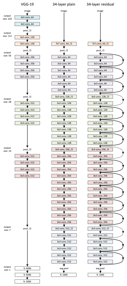
The image below shows a comparison between VGG-19, a convolutional neural network architecture without residual connections, and one with residual connections – ResNet34.

In this notebook we’ll also be showing how to use torchvision to handle datasets that are not part of torchvision.datasets. Specificially we’ll be using the 2011 version of the CUB200 dataset. This is a dataset with 200 different species of birds. Each species has around 60 images, which are around 500×500 pixels each. Our goal is to correctly determine which species an image belongs to – a 200-dimensional image classification problem.
As this is a relatively small dataset – ~12,000 images compared to CIFAR10’s 60,000 images – we’ll be using a pre-trained model and then performing transfer learning using discriminative fine-tuning.
Note: on the CUB200 dataset website there is a warning about some of the images in the dataset also appearing in ImageNet, which our pre-trained model was trained on. If any of those images are in our test set then this would be a form of “information leakage” as we are evaluating our model on images it has been trained on. However, the GitHub gist linked at the end of this article states that only 43 of the images appear in ImageNet. Even if they all ended up in the test set this would only be ~1% of all images in there so would have a negligible impact on performance.
We’ll also be using a learning rate scheduler, a PyTorch wrapper around an optimizer which allows us to dynamically alter its learning rate during training. Specifically, we’ll use the one cycle learning learning rate scheduler, also known as superconvergnence, from this paper and is commonly used in the fast.ai course.
Data Processing
As always, we’ll start by importing all the necessary modules. We have a few new imports here:
lr_schedulerfor using the one cycle learning rate schedulernamedtuplefor handling ResNet configurationsosandshutilfor handling custom datasets
